Implicit Restarting

  A restarting alternative has been proposed by Saad based upon the polynomial  acceleration scheme developed by Manteuffel [27] for the iterative solution of linear systems. Saad [39] proposed to restart the factorization with a vector that has been preconditioned so that it is more nearly in a k-dimensional invariant subspace of interest. This preconditioning takes the form of a polynomial in ${\bf A}$ applied to the starting vector that is constructed to damp unwanted components from the eigenvector expansion. An iteration is defined by a repeatedly restarting until the current Arnoldi factorization contains the desired information. Saad's ideas are closely related to techniques developed for the Lanczos process by Paige [35], Cullum and Donath [6], and Golub and Underwood [17]. The first example of a restarted Lanczos method that we are aware of was proposed by Karush [19].

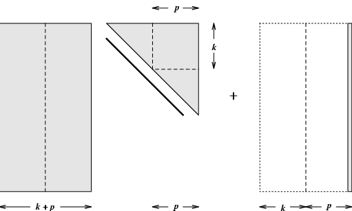
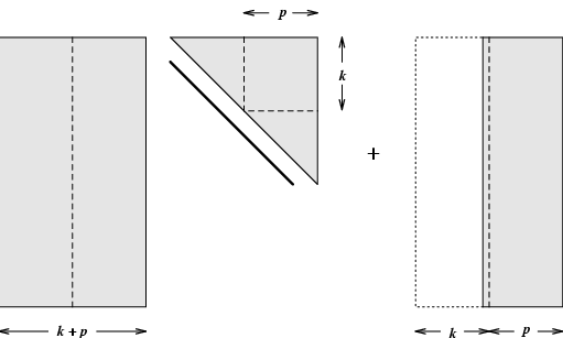
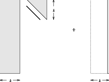
The ARPACK software is based upon another approach to restarting that offers a more efficient and numerically stable formulation. This approach called implicit restarting     is a technique for combining the implicitly shifted QR scheme with a k-step Arnoldi or Lanczos factorization to obtain a truncated  form of the implicitly shifted QR-iteration. The numerical difficulties and storage problems normally associated with Arnoldi and Lanczos processes are avoided. The algorithm is capable of computing a few (k) eigenvalues with user specified features such as largest real part or largest magnitude using storage. No auxiliary storage is required. The computed Schur basis vectors for the desired k-dimensional eigen-space are numerically orthogonal to working precision. The suitability of this method for the development of mathematical software stems from this concise and automatic treatment of the primary difficulties with the Arnoldi/Lanczos process.

Implicit restarting provides a means to extract interesting information from large Krylov subspaces while avoiding the storage and numerical difficulties associated with the standard approach. It does this by continually compressing the interesting information into a fixed size k-dimensional subspace. This is accomplished through the implicitly shifted QR mechanism. An Arnoldi factorization of length m = k+p

(2)

is compressed to a factorization  of length k that retains the eigen-information of interest. This is accomplished using QR steps to apply p shifts implicitly. The first stage of this shift process results in   where , , and Each is the orthogonal matrix associated with the shift used during the shifted QR algorithm. Because of the Hessenberg structure of the matrices , it turns out that the first k-1 entries of the vector are zero (i.e. ). This implies that the leading k columns in equation (4.4.2) remain in an Arnoldi relation. Equating the first k columns on both sides of (4.4.2) provides an updated k-step Arnoldi factorization

(4)

with an updated residual of the form . Using this as a starting point it is possible to apply p additional steps of the Arnoldi process to return to the original m-step form.

Each of these shift cycles results in the implicit application of a polynomial  in ${\bf A}$ of degree p to the starting vector.

The roots of this polynomial are the shifts used in the QR process and these may be selected to filter    unwanted information from the starting vector and hence from the Arnoldi factorization. Full details may be found in [44].

The choice of shifts  and hence construction of the polynomial is motivated by the fact that if the starting vector where ,then , and thus will provide an orthonormal basis for the invariant subspace Moreover, the spectrum of will be the desired eigenvalues:

  

Figure 4.4: Algorithm 3: An Implicitly Restarted Arnoldi Method (IRAM).

Input: ( ${\bf A}, {\bf V}, {\bf H}, {\bf f}$) with ${\bf A}{\bf V}_m = {\bf V}_m {\bf H}_m + {\bf f}_m {\bf f}e_m^T$, an $m$-step Arnoldi factorization;

For $\ell=1,2,3,...$ until $convergence$

(a3.2) Compute $\sigma({\bf H}_m)$ and select set of $p$ shifts $\mu_1, \mu_2 ,... \mu_p$

based upon $\sigma({\bf H}_m)$ or perhaps other information;

(a3.3) ${\bf Q} = {\bf I}_m$
(a3.4) For $j = 1,2,...,p$,


Factor $[ {\bf Q}_j, {\bf R}_j] = {\mbox qr}( {\bf H}_m - \mu_j {\bf I})$;
${\bf H}_m \leftarrow {\bf Q}_j^H {\bf H}_m {\bf Q}_j$; ${\bf Q} \leftarrow {\bf Q} {\bf Q}_j$;
End_For

(a3.5) $\hat{\beta}_{k} = {\bf H}_m(k+1,k);$ $\sigma_k = {\bf Q}(m,k);$

(a3.6) ${\bf f}_k \leftarrow {\bf v}_{k+1}\hat{\beta}_{k} + {\bf f}_m \sigma_k$;


(a3.7) ${\bf V}_k \leftarrow {\bf V}_m {\bf Q}(:,1:k); {\bf H}_k \leftarrow {\b f H}_m(1:k,1: k);$


(a3.8) Beginning with the $k$-step Arnoldi factorization ${\bf A}{\bf V}_k = {\bf V}_k {\bf H}_k + {\bf f}_k {\be e}_k^T$,
apply $p$ additional steps of the Arnoldi process
to obtain a new $m$-step Arnoldi factorization ${\bf A} {\bf V}_m = {\bf V}_m {\bf H}_m + {\bf f}_m {\bf e}e_m^T$ .

End_For

  ;

Figure 4.5: The set of rectangles represents the matrix equation of an Arnoldi factorization. The unshaded region on the right is a zero matrix of m-1 columns.

  

Figure 4.6: After performing m-k implicitly shifted QR steps on , the middle set of pictures illustrates The last p columns of are nonzero because of the QR iteration.

  

Figure 4.7: An implicitly restarted length k Arnoldi factorization results after discarding the last m-k columns.

The repeated update of the starting vector through implicit restarting is designed to enhance the components of this vector in the directions of the wanted eigenvectors and damp its components in the unwanted directions. If has an expansion as a linear combination of eigenvectors of ${\bf A}$, the effect of this polynomial restarting   is illustrated as follows:

If the same polynomial (i.e. the same shifts) were applied each time, then after iterations, the j-th original expansion coefficient would be essentially attenuated by a factor

where the eigenvalues have been ordered according decreasing values of . The leading k eigenvalues become dominant in this expansion and the remaining eigenvalues become less and less significant as the iteration proceeds. Adaptive choices of shifts can further enhance the isolation of the wanted components in this expansion. Hence, the wanted eigenvalues are approximated better and better as the iteration proceeds.

The basic iteration is listed in Figure 4.4 as Algorithm 3 and the diagrams in Figures 4.5--4.7 describe how this iteration proceeds schematically. In Algorithm 3 and in the discussion that follows, the notation denotes the leading submatrix of

We illustrate a typical polynomial that was constructed during an iteration on a matrix ${\bf A}$ that is a small example of a turbine model. The goal was to compute the five eigenvalues of largest real part of this order 375 matrix. The surface shown in Figure 4.8 is the plotted over a region containing the spectrum of ${\bf A}$. Here, is the product of all of the filter polynomials constructed during the course of the iteration. The degree of is around 600 and this would be quite challenging to apply directly. The ``+" signs are the eigenvalues of ${\bf A}$ in the complex plane and the contours are the level curves of . The circled plus signs are the converged eigenvalues including two complex conjugate pairs and on real root of largest real part. Observe how well the the location of the unwanted portion of the spectrum was determined and damped during the course of the iteration. The figure illustrates that this method can isolate desired eigenvalues on the ``boundary" of the spectrum even though they may be quite close to other eigenvalues. However, when the clustering becomes pronounced, it will be very difficult to achieve this.

  

Figure 4.8: Total filter polynomial from an IRA iteration.

Observe that if m = n then and this iteration is precisely the same as the Implicitly Shifted QR iteration. Even for m < n, the first k columns of and the Hessenberg submatrix are mathematically equivalent to the matrices that would appear in the full Implicitly Shifted QR iteration using the same shifts In this sense, the Implicitly Restarted Arnoldi method may be viewed as a   truncation of the Implicitly Shifted QR iteration. See [23] for details on a connection with subspace iteration   and the QR algorithm.  The fundamental difference is that the standard Implicitly Shifted QR iteration selects shifts to drive subdiagonal elements of to zero from the bottom up while the shift selection in the Implicitly Restarted Arnoldi method is made to drive subdiagonal elements of to zero from the top down.

Important implementation details concerning the deflation  (setting to zero) of subdiagonal elements of and the purging  of unwanted but converged Ritz values are beyond the scope of this discussion. However, these details are extremely important to the success of this iteration in difficult cases. Complete details of these numerical refinements may be found in [26,22].

The above iteration can be used to apply any known polynomial restart. If the roots of the polynomial are not known there is an alternative implementation that only requires one to compute where is the desired degree p polynomial. A sequence of Householder transformations may developed to form a unitary matrix such that and is upper Hessenberg. The details which follow standard developments for the Implicitly Shifted QR iteration will be omitted here.

A shift selection strategy that has proved successful in practice and is used as the default in ARPACK is called the ``Exact Shift Strategy". In this strategy, one computes and sorts this into two       disjoint sets and The k Ritz values in the set are regarded as approximations to the ``wanted" eigenvalues  of ${\bf A}$ , and the p Ritz values in the set are taken as the shifts . An interesting consequence (in exact arithmetic) is that after Step (a3.4) above, the spectrum of in Step (a3.6) is and the updated starting vector is a particular linear combination of the k Ritz vectors associated with these Ritz values. In other words, the implicit restarting scheme with exact shifts provides a specific selection of expansion coefficients for a new starting vector as a linear combination of the current best estimates (the Ritz vectors) for wanted eigenvectors. This implicit scheme costs p rather than the k+p matrix-vector products the explicit scheme would require. Thus the exact shift strategy can be viewed both as a means to damp unwanted components from the starting vector and also as directly forcing the starting vector to be a linear combination of wanted eigenvectors. See [23,44] for information on the convergence of IRAM and [3,45] for other possible shift strategies for Hermitian The reader is referred to [25,33] for studies comparing implicit restarting with other schemes.